Aeroelastic Simulations
Flutter analysis of an AGARD 02 wing
The occurence of strong nonlinearities in the flow field, such as for
example shock waves or flow separation, requires for the adoption of
CFD methods for aeroelastic stability assessment in the transonic
regime. However, it can be observed that while the steady flow fields
is highly nonlinear, the same does not hold for the unsteady loads
which influences the aeroelastic stability. The latter can be often
considered with an high level of accuracy as linear [31,32].
In any case, nonlinearities in the flow equations require to study the
stability of each flight configuration independently. To speed up the
analysis, especially when a large number of configurations needs to be
tested, a linearized model of the unsteady aerodynamic forces is
extracted from CFD solutions by evaluating the aerodynamic response to
relevant modal deformations of the structure, without the need of
performing a fully coupled nonlinear analysis for each test condition.
The result of the linearisation is a Reduced Order Model (ROM) for
aerodynamic unsteady forces. It is therefore possible to use CFD-ALE
time marching solutions as a sort of "numerical experiments" for the
extraction of the dynamics of the flow field. To this purpose it is
necessary to run a set of specified simulation with imposed wall
boundary movements, choosing a simple excitation method which requires
a reasonable computational cost but permits a good identification of
the principal dynamics of aerodynamic forces Fa [27].
A linear modal representation of the structure is used, as it is usually done in classic aeroelastic analysis [20]. In this case, the classical flutter problem can be stated as follows: find the dynamic pressure q which gives rise to unstable free movements for a given (linear) elastic structure represented in modal form as


A linear modal representation of the structure is used, as it is usually done in classic aeroelastic analysis [20]. In this case, the classical flutter problem can be stated as follows: find the dynamic pressure q which gives rise to unstable free movements for a given (linear) elastic structure represented in modal form as
where M, C,
K
are respectively the modal mass, damping and stiffness
matrices, and Fa are the generalized aerodynamic
forces associated with
each mode. As an application to the CA scheme outlined above, the Agard
445.6 deformable wing test case is now considered. Experimental results
for the wind tunnel tests can be found in the report [28]. The tested
wing presents a clear drop of the flutter velocity in transonic flow
conditions, so it has been taken by many authors as the reference case
to assess the quality of the transonic
flutter prediction [29,30]. For numerical flutter computations
only the first two modes are taken into account, where the first is a
bending mode while the second is a torsional one (cf. Figure 11 and 12), as
they
are deemed sufficient to predict the onset of flutter instability. A
three-dimensional tetrahedral fluid mesh, containing 22014 nodes is
used as the aerodynamic grid. The input signal given to the aerodynamic
system, represented by the modal deformation amplitude imposed to the
boundary of fluid grid, is of the form:
where  is the highest reduced frequency
of interest and
is the highest reduced frequency
of interest and  is the amplitude of
the i-th mode (~
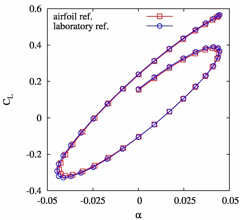
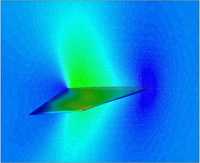
0.01 here). Fig. 16 shows the maximum deformations reached during the
simulation and corresponding Mach contours for the first and second
modes. The simulation with imposed wall boundary movements along the
first and the second mode allows to compute the real and imaginary part
of the frequency response matrix of the generalized aerodynamic forces.
These results are then used to compute the flutter onset point.
Flutter analysis are performed for several Mach numbers, namely in the
subsonic, transonic and supersonic regimes. The plot shows the flutter
speed index, defined as
is the amplitude of
the i-th mode (~
0.01 here). Fig. 16 shows the maximum deformations reached during the
simulation and corresponding Mach contours for the first and second
modes. The simulation with imposed wall boundary movements along the
first and the second mode allows to compute the real and imaginary part
of the frequency response matrix of the generalized aerodynamic forces.
These results are then used to compute the flutter onset point.
Flutter analysis are performed for several Mach numbers, namely in the
subsonic, transonic and supersonic regimes. The plot shows the flutter
speed index, defined as
is the highest reduced frequency
of interest and is the amplitude of
the i-th mode (~
0.01 here). Fig. 16 shows the maximum deformations reached during the
simulation and corresponding Mach contours for the first and second
modes. The simulation with imposed wall boundary movements along the
first and the second mode allows to compute the real and imaginary part
of the frequency response matrix of the generalized aerodynamic forces.
These results are then used to compute the flutter onset point.
Flutter analysis are performed for several Mach numbers, namely in the
subsonic, transonic and supersonic regimes. The plot shows the flutter
speed index, defined as is the frequency of the torsional mode and
  is
the mass ration. The result of the numerical
analysis are summarized in Figure
is
the mass ration. The result of the numerical
analysis are summarized in Figure