Dynamic Simulations of a Flap Opening
The motion of the grid is carried out resorting to edge swapping, node insertion, node deletion and grid deformation.
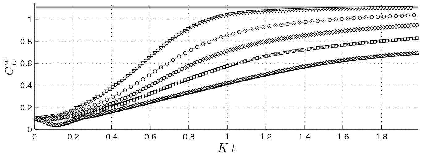
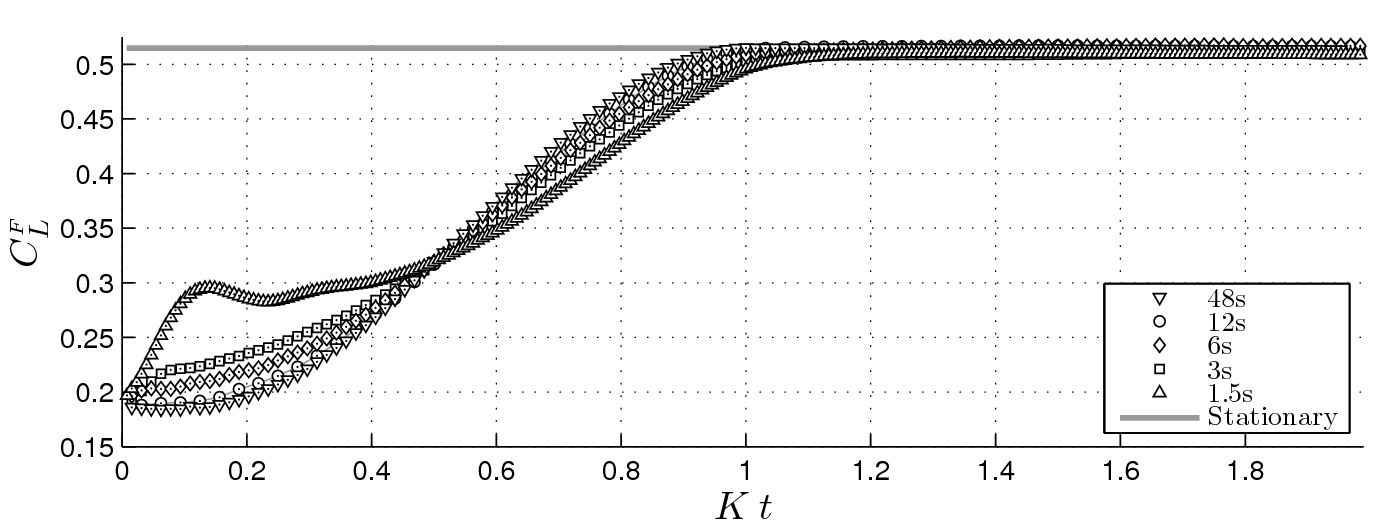
In Figure 8 and 9 results for a fowler flap
extraction problem are shown for the N1WC2F1 airfoil.
The motion of the flap airfoil is imposed through the sinusoidal law xflap(t)=x0 + 0.5(xf-x0)(1-cos( pi K t )) and similarly for the
flap angle delta. x0 and xf are the distances of
the flap nose from the main airfoil one, respectively at the initial
time t0 and at the final time tex.
At the time t=tex
the flap is completely opened, thus no further modifications of the
geometry occurs for t > tex.
The geometry parameters are gathered in Table 2; the reader is referred
to Ref. 33 for the definition of the
airfoil geometry.
In Movie 7 the domain triangulation during the extraction of a flap is shown. Mesh movement is performed resorting to the complete adaptation procedure and the regularity of the mesh is very high, note that the airfoil is not translating inside a fixed domain. It is to be noted also that such peculiar movement can not be properly performed without resorting to node insertion and deletion technique due to the large variation in size of the gap between the airfoils.
Dynamic simulations have been performed for different extraction times tex=2/K ranging from 1.5 to 48, see Figure 8 and 9. The free stream flow has a an angle of attack alpha=0.1° and a Mach number M=0.55. Computation has been performed using the first order Roe fluxes. It can be observed that the flap lift coefficient CLF(t) curves overlap fairly well if the adimensional time t is scaled with tex/2. The lift coefficient is very close to the stationary value at Kt=1, namely, when the extraction is completed. The above does not hold for the main body lift coefficient CLw(t). The CL curves of Figure 8 and 9., for both the main body and the flap, approach the quasi-static behaviour as the extraction time is increased; transient oscillations appear for rapid movement of the flap surface.
|
|
|||||||||||||
In Movie 7 the domain triangulation during the extraction of a flap is shown. Mesh movement is performed resorting to the complete adaptation procedure and the regularity of the mesh is very high, note that the airfoil is not translating inside a fixed domain. It is to be noted also that such peculiar movement can not be properly performed without resorting to node insertion and deletion technique due to the large variation in size of the gap between the airfoils.
 Movie 7. Flap
extraction, computational mesh, close-up. Movie 7. Flap
extraction, computational mesh, close-up. |
||
| Click here to download high
quality |
Dynamic simulations have been performed for different extraction times tex=2/K ranging from 1.5 to 48, see Figure 8 and 9. The free stream flow has a an angle of attack alpha=0.1° and a Mach number M=0.55. Computation has been performed using the first order Roe fluxes. It can be observed that the flap lift coefficient CLF(t) curves overlap fairly well if the adimensional time t is scaled with tex/2. The lift coefficient is very close to the stationary value at Kt=1, namely, when the extraction is completed. The above does not hold for the main body lift coefficient CLw(t). The CL curves of Figure 8 and 9., for both the main body and the flap, approach the quasi-static behaviour as the extraction time is increased; transient oscillations appear for rapid movement of the flap surface.
 Movie 8. Flap extraction, entropy loss, Mach and streamlines. |
||
|
Click here to download high quality
|