Pitching NACA 0012 Airfoil
NACA 0012 airfoil translating and pitching inside a domain. Instead of using the standard solid body reference, the airfoil is moving inside the computational domain of still air. The motion is performed thanks to mesh deformation, swapping and node removal/deletion. The ALE formulation allows to avoid any interpolation of the solution.
A two-dimensional example of
the proposed strategy is given in Figure 5,
where the grid used in the computation of the aerodynamic behaviour of
an oscillating NACA0012 airfoil flying at Mach number 0.75 is
also depicted. This test case is often used in the assessment of
CFD
code over moving domain for it provides a two-dimensional
representation of a pitching rotor blade.
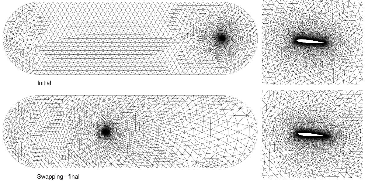
Instead of considering an airfoil that is oscillating in fluid in motion, which would require only a minor, local, deformation of the grid, a still fluid is assumed in which the airfoil both oscillates and translates to the left to cover a distance equal to 65 airfoil chords, which is approximatively the displacement of the blade tip during a single revolution. In the second situation, the domain boundaries are massively displaced and standard grid movement techniques cannot be used. However, it is still possible to modify the computational mesh without re-meshing the whole domain by resorting to successive steps of grid deformation and edge-swapping. Grid deformation is used to move the grid node to their new positions, whereas edge-swapping is used to break the element connectivity to let element literally flow around the airfoil. The resulting grid is depicted in Figure 5(bottom), where the grid quality as well as the higher spatial resolution close to the airfoil are preserved from the initial grid.
Since the number of grid nodes remains constant as the simulation progresses, the computational grid at a given time level can be described in terms of the corresponding nodes at the previous time level. In other words, the new grid is obtained via a suitable deformation of a fictitious grid defined by the current element-node connectivity and the previous node positions. It is therefore possible to obtain the solution at the current time level by employing standard ALE techniques, thus avoiding the need of re-interpolating the solution. Hence, standard BDF techniques can be implemented very easily.
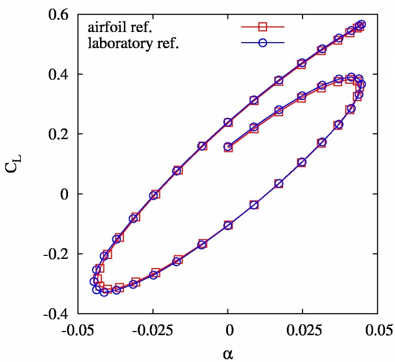
5 reports the results of the CFD simulations. Standard ALE results refer to computations performed on an airfoil-centered reference, with the airfoil varying only its pitch in time [1]. Numerical simulations obtained with the present method are instead performed on a fixed grid (laboratory reference) through which the airfoil is translating (and oscillating) at Mach number 0.755. Results in terms of lift coefficient against incidence are reported in Figure 6.
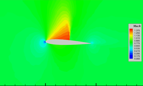
In Movie 1 the Mach number field close to the airfoil is shown. Because of the airfoil pitching motion two shockwaves are alternatively generated and destroyed above and below the airfoil.
Instead of considering an airfoil that is oscillating in fluid in motion, which would require only a minor, local, deformation of the grid, a still fluid is assumed in which the airfoil both oscillates and translates to the left to cover a distance equal to 65 airfoil chords, which is approximatively the displacement of the blade tip during a single revolution. In the second situation, the domain boundaries are massively displaced and standard grid movement techniques cannot be used. However, it is still possible to modify the computational mesh without re-meshing the whole domain by resorting to successive steps of grid deformation and edge-swapping. Grid deformation is used to move the grid node to their new positions, whereas edge-swapping is used to break the element connectivity to let element literally flow around the airfoil. The resulting grid is depicted in Figure 5(bottom), where the grid quality as well as the higher spatial resolution close to the airfoil are preserved from the initial grid.
Since the number of grid nodes remains constant as the simulation progresses, the computational grid at a given time level can be described in terms of the corresponding nodes at the previous time level. In other words, the new grid is obtained via a suitable deformation of a fictitious grid defined by the current element-node connectivity and the previous node positions. It is therefore possible to obtain the solution at the current time level by employing standard ALE techniques, thus avoiding the need of re-interpolating the solution. Hence, standard BDF techniques can be implemented very easily.
5 reports the results of the CFD simulations. Standard ALE results refer to computations performed on an airfoil-centered reference, with the airfoil varying only its pitch in time [1]. Numerical simulations obtained with the present method are instead performed on a fixed grid (laboratory reference) through which the airfoil is translating (and oscillating) at Mach number 0.755. Results in terms of lift coefficient against incidence are reported in Figure 6.
 Movie 1. Mach number contour obtained translating the airfoil at M=0.755, using mesh deformation and edge swapping. |
||
| Click
here to download high
quality |
In Movie 1 the Mach number field close to the airfoil is shown. Because of the airfoil pitching motion two shockwaves are alternatively generated and destroyed above and below the airfoil.